

Processor applies each processing step as a layer, altering the shape of your spectrum, but leaving the original spectral data untouched. The Processing History records each layer along with its associated parameters, like phase angles, baseline breakpoints and linewidth adjustments. You can review the layers, edit them, and even remove them if necessary, restoring your spectrum to an earlier state.
When you import a processed spectrum, all processing that you have
performed in other software appears in the Processing History as a layer
called External Processing; the details of the External Processing layer
indicate the format from which the processed data was imported. The
External Processing layer is not reversible, and cannot be removed. If
you need to work with the spectrum as it appeared before processing in
other software, import the raw data (fid,
.jdf, .fid) directly.
Line broadening is a mathematical operation that multiplies your fid by an exponential function before the fid is Fourier transformed. Line broadening effectively increases the linewidth in your spectrum while averaging out instrument noise.
You may not need to apply line broadening to every spectrum. If you choose to use line broadening, apply it after phase correction and baseline correction.
While importing a spectrum, you may choose to have Processor automatically apply line broadening of 0 to 1000 Hz. After importing a spectrum, you can apply line broadening manually. In either case, a Line Broadening layer appears in the Processing History; you can remove the layer if necessary.
| Menu Location | Processing > Line Broadening... |
| Icon |
|
How do I apply line broadening to my spectrum?
-
Switch to Line Broadening mode.
-
Enter a value between 0 and 1000 Hz.
-
Click the Accept button.
Tips and Tricks
-
If you intend to apply shim correction to your spectrum, you can add line broadening at the same time. See “Shim Correction” for details.
-
To apply line broadening to more than one spectrum at a time, use the “Batch Process” tool.
Phase correction lets you correct phase shifts that may have occurred during data acquisition. You can recognize phase shifts in a spectrum as an asymmetric baseline on either side of peaks and peak clusters in the spectrum. In some cases, you may see whole peaks inverted, pointing down from the baseline instead of up, while extreme phase shifts may also add a periodic oscillation or "rolling" to the baseline.
Most spectra require some degree of phase correction. Phase should be adjusted before applying baseline correction or shim correction.
While importing a spectrum, you may choose to have Processor automatically apply phase correction. After importing a spectrum, you can apply automatic or manual phase correction. In either case, a Phase Correction layer appears in the Processing History; you can remove the layer if necessary.
| Menu Location | Processing > Phase Correction... |
| Icon |
|
How do I apply phase correction to my spectrum?
-
Switch to Phase Correction mode.
-
Automatic: Click the Auto button to have Processor automatically calculate phase angles. Review the spectrum after automatic phase correction to ensure that the results are acceptable. If necessary, you can use the manual controls to adjust the phase angles before accepting them.
-
Manual: Click and drag the Zero-order Phase and First-order Phase sliders, or type angles in the boxes beside each slider. Use the Fine Tune checkbox to adjust the spectrum more gradually while moving the sliders.
-
Click the Accept button to apply your changes, or click the Cancel button to discard them.
Tips and Tricks
-
Properly phase all of your spectra, as good phase correction is essential to accurately analyzing your data using Chenomx NMR Suite. Your spectrum is properly phased when its baseline is a smooth curve (or line) across the entire width of the spectrum.
-
A good strategy for manual phasing is to pick a peak on the far right side of your spectrum, adjust the Zero-order phase until the baseline on either side of the peak lines up, then pick a peak on the far left side and adjust the First-order phase in the same way. Repeat this process until the entire spectrum is well-phased.
-
Only phase your spectrum once. If you do not like the results of phase correction, undo it or remove it using the Processing History, then try again.
-
Always phase your spectrum before applying baseline correction or any other processing layers.
-
Select one of the phase angle controls, and use the arrow keys to make fine adjustments to the phase angle. The arrow keys adjust in increments of 0.15° normally, and in 0.01° increments when the Fine Tune checkbox is selected.
-
In spectra of aqueous samples, the water peak may be distorted relative to the rest of the spectrum; do not use the water peak to determine phase correction. Instead, try to obtain smooth baseline curves to either side of the water peak.
-
During a phase correction session, you can clear your current adjustments by clicking the Reset button. After you have accepted your changes, you can clear previous adjustments through the Processing History panel.
-
To apply phase correction to more than one spectrum at a time, use the “Batch Process” tool.
Baseline correction lets you remove distortions in the baseline of the spectrum. You can recognize distorted baselines as a net curvature or slant of the regions of your spectrum that contain no signal ("noise" regions). Common forms of baseline distortions include "smiles" (outer regions of the spectrum turned up), "frowns" (outer regions of the spectrum turned down) and "wings" (left and right edges of the spectrum turned up or down, with the middle region flat). If you notice a periodic oscillation or "rolling" of the baseline, check the phase correction of your spectrum before proceeding with baseline correction.
Most spectra require some degree of baseline correction, particularly if you need accurate quantification in Profiler. Apply baseline correction after phase correction, but before shim correction.
While importing a spectrum, you may choose to have Processor automatically apply either simple linear baseline correction (drift correction) or a cubic spline baseline correction based on automatically-determined breakpoints. After importing a spectrum, you can apply automatic or manual baseline correction. In either case, a Baseline Correction layer appears in the Processing History panel; you can remove this layer if necessary.
For more direct control over the baseline correction applied to your spectrum, you can specify breakpoints manually.
| Menu Location | Processing > Baseline Correction... |
| Icon |
|
How do I apply baseline correction to my spectrum?
-
Switch to Baseline Correction mode.
-
Select the type of baseline to be performed from the Automatic BaseLine Correction pull-down menu. Four different types of baseline are available:
-
Linear (Drift): Simple drift correction by passing a baseline through the edges of the spectrum.
Or
Chenomx Spline: Cubic-spline-based baseline adjustment.
Or
Whitaker Spline: Whitaker filter followed by cubic interpolation of equally-spaced points.
Or
BXR Spline: BXR algorithm followed by cubic interpolation of equally-spaced points.
-
You can control the number of automatically generated breakpoints, and in the case of the Whitaker anx BXR splines, the smoothness of the produced baseline by clicking on the engineer wheel icon next to the pull-down menu.
-
Manual: Click on the spectrum to set breakpoints for a cubic spline fit. Click and drag existing breakpoints (including the endpoints) to move them. Hold down Control or Command to place breakpoints anywhere in the spectrum, instead of directly on the spectrum line itself. Hold down Shift while clicking on an existing breakpoint to delete it. Hold down Shift while delimiting a box inside the spectrum to delete multiple breakpoints at once.
-
Click the Accept button to apply your changes, or click the Cancel button to discard them.
Tips and Tricks
-
Only apply baseline correction after you are satisfied with the phase correction in your spectrum.
-
Even if you intend to manually adjust baseline correction, you may find it helpful to use the Auto Linear function first. Auto Linear lets Processor first locate the "natural" endpoints of the spectrum, giving you a useful starting point for any more complex baseline fit.
-
When setting breakpoints, be aware of the amount of curvature in the area you are trying to fit. You need to set more breakpoints to fit regions with very strong curvature, such as the areas near the water peak, than you would for a relatively flat region.
-
To apply baseline correction to more than one spectrum at a time, use the “Batch Process” tool.
Shim correction is a method of reconstructing an ideal spectrum by removing lineshape distortions based on the shape of a reference peak. To successfully apply shim correction to a spectrum, you need to find a single, isolated peak, well-separated from the signals in the rest of the spectrum. If you have added DSS or TSP to your sample, the methyl signal from either of these is an ideal choice.
Shim correction is a linear process, using direct and inverse Fourier transforms, so quantitative relationships among compounds in the spectrum remain intact. Applying shim correction to a spectrum assumes that all lineshapes in the spectrum are affected by systematic distortions in the same way.
Many spectra can benefit from the use of shim correction, but it is not required. It is particularly useful in reducing the effects of varying shimming techniques, or when you need accurate quantification from regions with strong overlap of signals.
You need to apply shim correction manually after you have imported your spectrum. After you have applied shim correction, a Shim Correction layer appears in the Processing History panel; you can remove this layer if necessary.
| Menu Location | Processing > Shim Correction... |
| Icon |
|
How do I apply shim correction to my spectrum?
-
Switch to Shim Correction mode.
-
Zoom in to the highlighted peak in the Spectrum Graph. If it is not properly fit to the peak that you are targeting for shim correction, adjust its fit as necessary.
-
If you are using DSS or TSP as your target peak, select the Use DSS/TSP Satellites check box. Otherwise, clear the check box.
-
Enter the desired target linewidth.
-
Click the Accept button to apply your changes, or click the Cancel button to discard them.
Tips and Tricks
-
Only apply shim correction after you are satisfied with the phase correction and baseline correction in your spectrum.
-
The target linewidth text box initially contains the native linewidth of your spectrum, based on your CSI definition.
-
Choosing a target linewidth larger than the native linewidth in your spectrum is equivalent to applying line broadening. Choosing a value smaller than the native linewidth may provide some resolution enhancement, at the expense of a reduced signal-to-noise ratio and possible spectral artifacts.
-
To apply shim correction to more than one spectrum at a time, use the “Batch Process” tool.
| Menu Location | Processing > Region Deletion... |
| Icon |
|
In many spectra of biofluids or cell extracts, the solvent peak (typically water) may be very large. In some cases, it is so large that seeing any other peaks while completely zoomed out is difficult. Region deletion is a simple processing layer that masks data points within a specified frequency range. It is designed to prevent the height of the solvent peak from dominating the vertical range of the spectrum display.
Using region deletion to remove the solvent peak is optional. Ensure that no peaks of interest occur close to the solvent peak before you apply region deletion, as such peaks may be masked by the region deletion layer.
While importing a spectrum from an aqueous sample, you may choose to have Processor automatically apply region deletion to the water peak. A Region Deletion layer appears in the Processing History panel; you can remove this layer if necessary.
How do I apply region deletion to my spectrum?
-
Switch to Region Deletion mode.
-
Enter the desired frequency range.
Or
Interact with the highlighted region in the graph to define the frequency range. You can drag the region by clicking inside of it, and expand or contract it by clicking on either edge of the region.
-
Click the Accept button to apply your changes, or click the Cancel button to discard them.
Tips and Tricks
-
Region deletion works best if it is applied after phase correction.
-
Region deletion is not only useful for removing the solvent peak from your spectrum; it can be used to remove other peaks and clusters as well.
-
To apply region deletion to more than one spectrum at a time, use the “Batch Process” tool.
| Menu Location | Processing > Reverse Spectrum |
| Icon |
|
Reverse spectrum reverses the order of the data points in your spectrum in the frequency domain, effectively flipping the spectrum horizontally.
You only need to use reverse spectrum with certain types of spectra from Bruker spectrometers. If you have trouble locating the CSI peak (when you have a CSI in the sample), or even making any sense of your spectrum after importing it, you may need to reverse the spectrum.
While importing a spectrum, you may choose to have Processor reverse the spectrum automatically. After importing a spectrum, you can reverse the spectrum manually. In either case, a Reverse Spectrum layer appears in the Processing History panel; you can remove this layer if necessary.
Tips and Tricks
-
If you notice that a spectrum from a particular spectrometer must be reversed, it is likely that all spectra from that instrument, especially those acquired with the same parameters, need to be reversed.
-
If it is necessary, apply Reverse Spectrum first, as other processing layers may be difficult to apply correctly when the spectrum is backwards.
-
To apply Reverse Spectrum to more than one spectrum at a time, use the “Batch Process” tool.
| Menu Location | Tools > Batch Process |
| Icon |
|
The Batch Process tool allows you to add, remove, and change
calibration and processing effects on multiple .cnx
files at the same time.
How do I add/remove/change processing effects for multiple spectra at once?
-
Click on Batch Process in the Tools menu.
-
Use the Add Files or Add Folder buttons as many times as desired to select one or more
.cnxfiles. These are the files that you'll be modifying. Click Next to move on to the next page. -
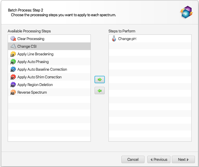
Choose to which calibrations and processing effects you would like to adjust by moving them from the list on the left to the list on the right. You can do this with the arrow buttons or simply by dragging and dropping them with the mouse. Click Next to continue.
-
You will now see a page of options for each calibration or effect that you have chosen. Adjust the options as you like, clicking Next after each.
-
On the final page, you'll see a summary of the changes that you are about to make. Once you are satisfied with them, click Finish and your changes will be applied.
How do I change the pH settings for multiple spectra at once?
The pH information of several samples/filenames can be read from an excel workbook and batch applied to a series of spectra.
-
Select Batch Process from the Tools menu. After choosing a set of files, select Change pH as a step to perform in the interface:
-
In the next interface that will appear, choose “From a custom list of file names and pH values”:
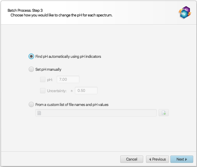
The provided excel workbook will be scanned for sample file names and pH information. The program will scan each tab/sheet of the provided excel workbook document (.xlsx) until it finds one that has a single row containing one of the mandatory valid column headers for BOTH the file names and their associated pH values.
The valid column header identifiers for the file names are: “name”, “sample”, or “filename”. The listed file names do not need the “.cnx” extension. If the file names are numerical in nature, and listed without their default “.cnx” extension, for instance: 10, 20,30, the cells must explicitly be formatted as Text inside Excel, not numbers.
The column containing pH information must be labeled “pH”, and nothing else.
Optionally, it is also possible to specify equidistant pH uncertainty ranges (+/-), with one of the following valid column labels: “∆pH”, “∆ pH”, “+/- pH”, “± pH”, or “pH uncertainty”. If this column is not provided, only the raw pH value of the listed samples will be changed to their listed values.
Once a row with all valid column headers have been found, the rest of the excel sheet will be read from the following row on and the information (filenames and pH values) will be extracted from their corresponding columns.
Tips and Tricks
-
The effects and calibrations that you apply with this tool are identical to the ones you can apply manually in Processor. You can read more detailed descriptions of each of them in other sections of this document.
-
You can check to see if your changes were applied correctly by opening your any of your newly batch processed spectra in Processor and inspecting its Processing History.