

Manual Profiling can involve a lot of effort in setting compound cluster positions and compound concentrations. Alternatively, you can use a semi-automated approach, or, with the introduction of version 10, a fully automated approach.
With the semi-automated approach, the first step consists of positioning compounds clusters on the spectra, followed by an automated concentration optimization based on those positions. Several rounds may be required.
First have Profiler fit cluster postions using the “First Step: Cluster positioning using Compound Snapper” tool and/or compound concentrations using the “Second Step: Concentration optimization using Fit Concentrations” for either the currently selected compound, a selection of compounds, or all compounds in the compound table.
Tips and Tricks
-
Use the Remember Selections feature to the mark compounds that can be reliably Autofit in your project. You can then restore the selection when working on subsequent spectra, allowing you to quickly autofit those compounds.
This feature allows for automatic positioning of peak clusters on the spectrum. It will essentially position peak clusters where their shape best match the experimental spectrum, independent of intensity.
Compound Snapper focuses on optimizing peak cluster locations, individually or in group, depending on the user’s selected cluster(s) or compound(s). Compound Snapper will not attempt to set or modify the concentration of compounds. This functionality automatically positions peak clusters on the spectrum at the location that best matches their global shape. If two or more clusters overlap within their allowed transform window, all possible combinations are analyzed.
As such, this feature is powerful, and will find the proper cluster combination, as sophisticated as it may be, that matches, according to shape, a relevant spectral region.
A snapping operation can either be performed on the original spectral line, or on the subtraction line, i.e. by considering the “left-over” signal from everything that has been fit already. It can also be done on a compound selected in the compound table and whose concentration has not been set already.
How to use Compound Snapper
-
Select one or several clusters from an individual compound, a single or several compounds at once from the compound table, right-click in your selection to bring a contextual menu, or choose 'Snap Compound' from the Compound Menu (main toolbar).
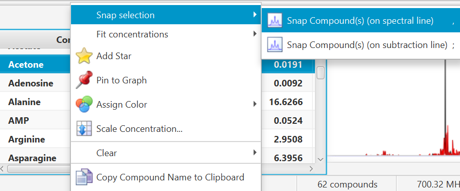
You can also use the keyboard shortcut comma (,) to snap clusters using the experimental spectrum line, or semi-colon (;) to snap clusters using the residual line instead (the residual line is calculated using everything that is already fit except for the clusters/compounds being snapped).
-
To snap all clusters resonating in a particular spectral region at once, first select the region with the Select Region tool (main tool bar), right-click and select “Find and Snap Peak Clusters in this Region”.
Once peak clusters have been positioned, compound concentrations can be fit and optimized using constrained penalized linear least squares, according to:
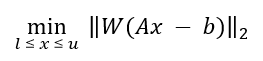
Where...
-
A is the model matrix made up the unscaled individual signatures of the compounds being fit. The current locations of the peak clusters are taken into account when the A matrix is calculated.
-
x is a vector made up all of the compound concentrations to be optimized. Each component of the vector, xi, is bounded between li (lower bound) and ui (upper bound). Non-negative restraints are imposed (li ≥ 0) since concentrations cannot be negative.
-
b is the spectral subtraction line, i.e. the experimental spectrum minus the contribution of all compounds part of the current profile that are not part of the optimization process. In other words, if a compound has been fit and his not part of the fitting process, its contribution is subtracted from the experimental spectrum before the process starts.
-
W is a weight vector, which is used to modulate the relative importance of each spectral point. Optionally, the algorithm can increase the weight of the points that are overfit though an iterative penalization process.
IMPORTANT NOTE: The optimization process will not modify the location of the peak clusters.
How to Fit Automatically
-
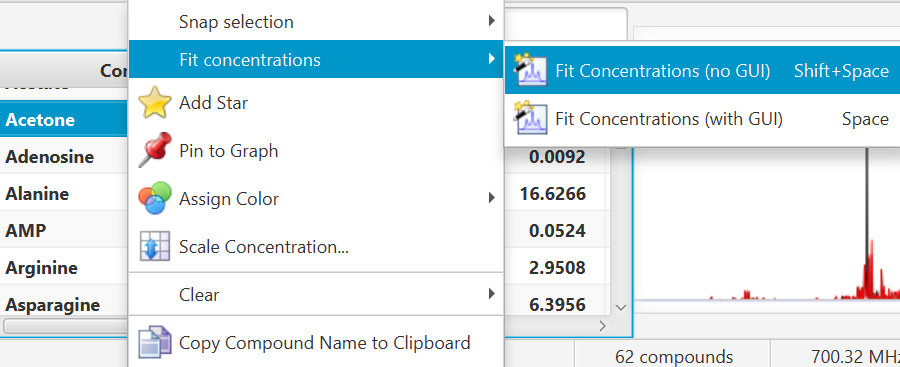
Right-click/control-click selected compounds in Profiler’s compound table, or on a selected spectral area.
Concentration Fitting can be performed without a GUI (graphical user interface) by using the Shift+Space bar keyboard shortcut, in which case it uses the default options and values stores in Profiler's preferences.
-
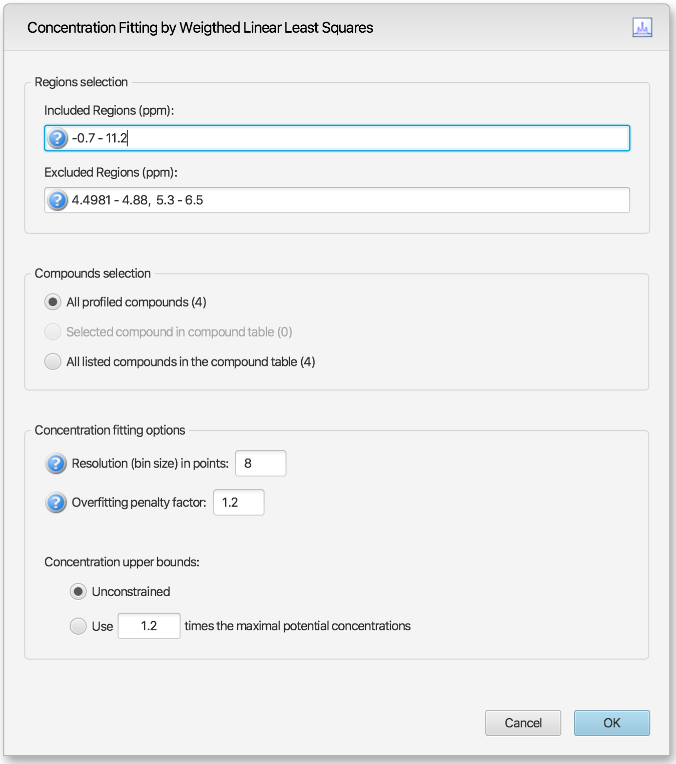
Alternatively, temporary settings can be entered via GUI (graphical user interface) using the space bar keyboard shortcut. The interface is composed of three main sections: Regions Selection, Compounds Selection, and Fitting options. The role of each section is described below. The application Preferences panel can be used to control and set all the default values appearing in the interface.
Regions Selection
-
Comma-separated list of spectral regions (in ppm units) to be included or excluded in the fit. Each component of the lists must include a lower and upper bound in ppm, separated by a dash. For instance, “0.8-2.3, 3.0-4.2” is a valid list.
-
The Included Regions input field displays the limits of the currently selected spectral region (as selected with the Select Region Tool), or of the selected clusters for an individual compound. If no region is currently selected, the Included Regions input field defaults to the entire spectrum.
-
The Excluded Regions input field will automatically include the region associated with the water peak. It is recommended that any peaks around the water region be excluded due to attenuation caused by water saturation. Similarly, the region associated with urea (5.4-6.0 ppm) should also be excluded if urea is present.
-
Excluded regions have prevalence over any included regions, i.e. any spectral point falling within any of the listed excluded regions will automatically be ignored during the fit.
Compound Selections
-
Users can optimize either all of the members of the current profile, all of the currently selected compounds in the compound table, or all of the currently listed compounds in the compound table. Note that compounds that do not have a single peak cluster within the participating spectral regions will not be considered for the fit. Their concentrations will not be changed.
Concentration Fitting Options
This group of options control the behavior of the optimization engine.
-
Resolution (bin size): The spectrum can be fit using either its full representation, or a binned representation of it. This parameter controls the number of spectral points per bin. Set this parameter to 1 for full resolution. However, it is highly recommended to use a binned representation if the peak cluster positions have not been optimized. Fitting at full resolution will require more memory and CPU time.
-
Overfitting penalty factor: The amount of overfitting can be limited by increasing the weights of the spectral points where overfitting occurs. This will effectively increase the importance of the spectral points where this occurs relative to the other ones, adding a penalty to pay for predicting points over the spectrum line. For a given spectral point, the square of the difference between the experimentally observed spectrum intensity and the predicted/calculated one will be multiplied by the factor specified in this field if the difference is negative. The weights are adjusted iteratively and up to 5 cycles of optimizations are performed if the specified penalty factor is >1.0.
-
Upper constraints: Non-negative constrained are used during the optimization process so that concentration values remain ≥ 0. Two different settings are offered to control their upper bounds. They can be set to be unlimited via the Unconstrained option, or limited according to their predetermined maximal potential concentration. The maximal potential concentration of a given compound is the highest concentration for which the compound signature would not exceed the experimental spectrum. Because of possible discrepancies between the compound library signatures and the experimental spectrum, mainly due to pH conditions, matrix effects, etc, the potential concentrations determined by Profiler may not be optimal and should only be regarded as guidelines. To give potential concentrations more wiggle room, potential concentrations can be pre-multiplied by a specified constant. The derived set of scaled potential concentration values will then be used as upper bounds.
IMPORTANT NOTE: The baseline is not modeled from the residuals at any stage. It is therefore crucial that the baseline be properly corrected prior to concentration fitting.
Related Topics
Version 10 of Chenomx NMR Suite introduces a new sophisticated, flexible and easy to use tool for automatic profiling of processed spectra.
Typically, when automatically fitting a spectrum, hundreds of variables (cluster positions and compounds concentrations) require optimization. Because compound concentrations are derived from existing peak cluster locations, and because peak clusters are allowed to be positioned within certain ranges (“transform windows”), several rounds of optimization are necessary to achieve a local or global minimum, i.e. a solution that reconstructs the experimental spectrum as best as possible.
Moreover, different mathematical solutions may recreate the experimental spectrum with similar degrees of fitness/fidelity. For this reason, the software can explore those solutions by repeating the fitting process for each individual input file as many times as the user chooses, and output a solution for each pass.
It is important to keep in mind that automatic profiling is purely a mathematical process that simply relies on a provided compound library. It does have not have the prior chemical knowledge of a human operator. COMPLETE Autofit should not be used blindly and fit results should be reviewed manually.
How to use COMPLETE Autofit
-
Open your processed CNX file within the Profiler Module.
-
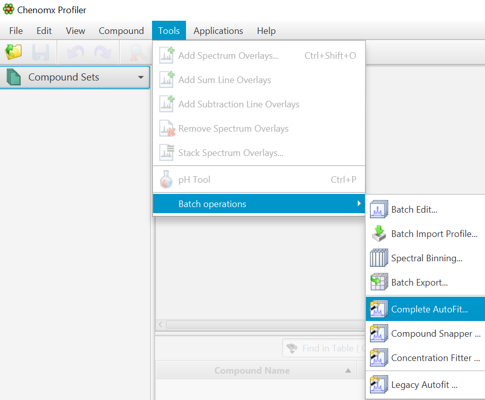
Go to Tools -> Batch Operations -> "COMPLETE Autofit"
-
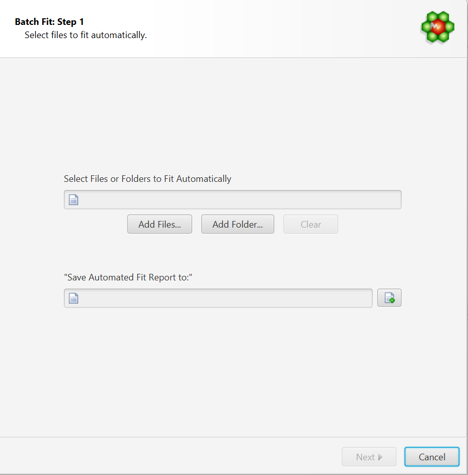
Select Files to Fit Automatically
-
Select Files or Folders to Fit Automatically: COMPLETE Autofit will do a complete profile of one, or several CNX files. Select your unprofiled CNX files here.
-
Save Automated Fit Report to: A fit report in the form of a tabulated separated value (tsv) file will be generated, with each input file and the sum of residuals associated with each fit attempt. Specify the destination and name of the report file here.
-
-
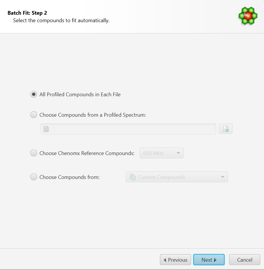
Select the Compounds to Fit Automatically. You can either:
-
Choose to fit all the compounds already profiled in each file. In this case, compounds must be already present in their profile and all of the compounds will be included in the fit operation.
-
Choose compounds from and already profiled spectrum. Note that it is possible to select only a subset of those in the interface’s next step.
-
Choose compounds from a Chenomx library
-
Choose compounds from a customized compound list defined in Library Manager.
IMPORTANT NOTE: DO NOT ATTEMPT TO FIT THE ENTIRE CHENOMX LIBRARY. THIS WILL RESULT IN OVERFITTING AND AN EXTREMELY LONG PROCESS. TARGET THE COMPOUNDS THAT SHOULD BE VISIBLE AND PRESENT FOR THE TYPE OF SAMPLES YOU HAVE.
-
-
Compound Selection Refinement
-
• Depending on your selection in the previous step, you may be presented with an option to further refine your compound selection. You can move compounds across list boxes to specify whether or not you want to include them in the fit.
-
• The checkbox option “Skip compounds that are already fit” is self-explanatory. It allows you to ignore compounds that are already fit. Their contribution will be calculated and taken in consideration to fit the reminder of the compounds, but their current state (cluster positions, concentrations) will not be modified.
-
-
Concentration Fitting Setup
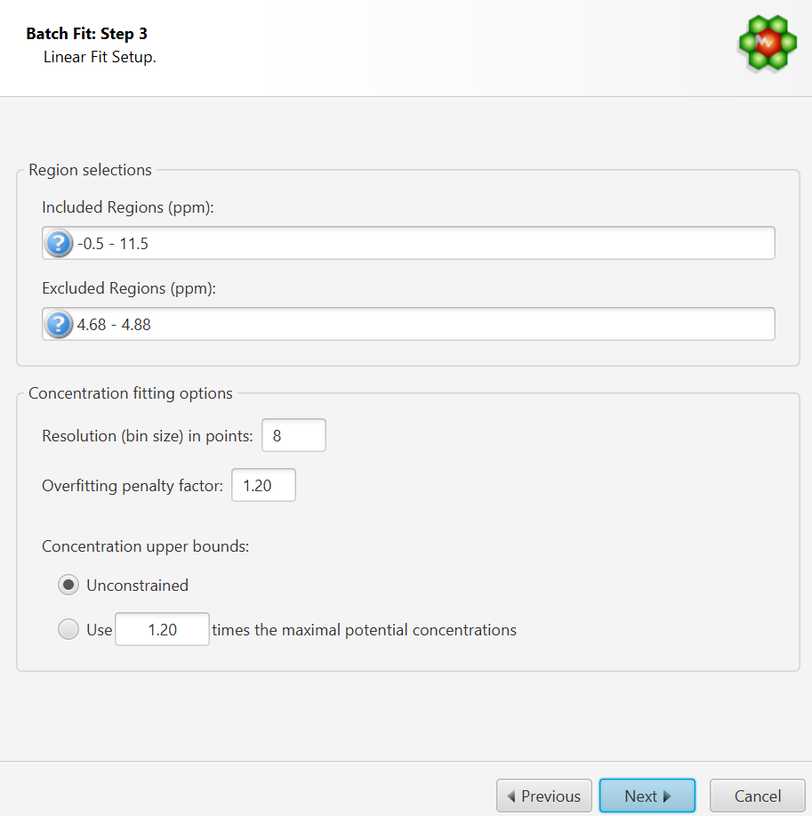
This interface is composed of two main sections: Regions Selection, and Concentration Fitting options. The role of each section is described below. The application Preferences panel can be used to control and set all the default values appearing in the interface.
-
Region Selection: Comma-separated list of spectral regions (in ppm units) to be included or excluded in the fit. Each component of the lists must include a lower and upper bound in ppm, separated by a dash. For instance, “0.8-2.3, 3.0-4.2” is a valid list.
-
The Included Regions input field displays the limits of the currently selected spectral region (as selected with the Select Region Tool). If no region is currently selected, the Included Regions input field defaults to the entire spectrum.
-
The Excluded Regions input field will automatically include the region associated with the water peak. It is recommended that any peaks around the water region be excluded due to attenuation caused by water saturation. Similarly, the region associated with urea (5.4-6.0 ppm) should also be excluded if urea is present.
Excluded regions have prevalence over any included regions, i.e. any spectral point falling within any of the listed excluded regions will automatically be ignored during the fit.
-
-
Concentration Fitting Options: This group of options control the behavior of the optimization engine.
-
Resolution(bin) size:
The spectrum can be fit using either its full representation, or a binned representation. This parameter controls the number of spectral points per bin. Set this parameter to 1 for full resolution. However, it is highly recommended to use a binned representation if the peak cluster positions have not been optimized. Fitting at full resolution will require more memory and CPU time.
-
Overfitting Penalty Factor:
The amount of overfitting can be limited by increasing the weights of the spectral points where overfitting occurs. This will effectively increase the importance of the spectral points where this occurs relative to the other ones, adding a penalty to pay for predicting points over the spectrum line. For a given spectral point, the square of the difference between the experimentally observed spectrum intensity and the predicted/calculated one will be multiplied by the factor specified in this field if the difference is negative. The weights are adjusted iteratively and up to 5 cycles of optimizations are performed if the specified penalty factor is >1.
-
Concentration Upper Bounds and Penalty Factor:
Non-negative constraints are used during the optimization process so that concentration values remain ≥ 0. Two different settings are offered to control their upper bounds. They can be set to be unlimited via the Unconstrained option, or limited according to their predetermined maximal potential concentration. The maximal potential concentration of a given compound is the highest concentration for which the compound signature would not exceed the experimental spectrum.
Because of possible discrepancies between the compound library signatures and the experimental spectrum, mainly due to pH conditions, matrix effects, etc, the potential concentrations determined by Profiler may not be optimal and should only be regarded as guidelines. To give potential concentrations more wiggle room, potential concentrations can be pre-multiplied by a specified constant. The derived set of scaled potential concentration values will then be used as upper bounds.
-
NOTE: It very important to note that the baseline is not modeled from the residuals at any stage. It is therefore crucial that the baseline be properly corrected prior to concentration fitting.
-
-
-
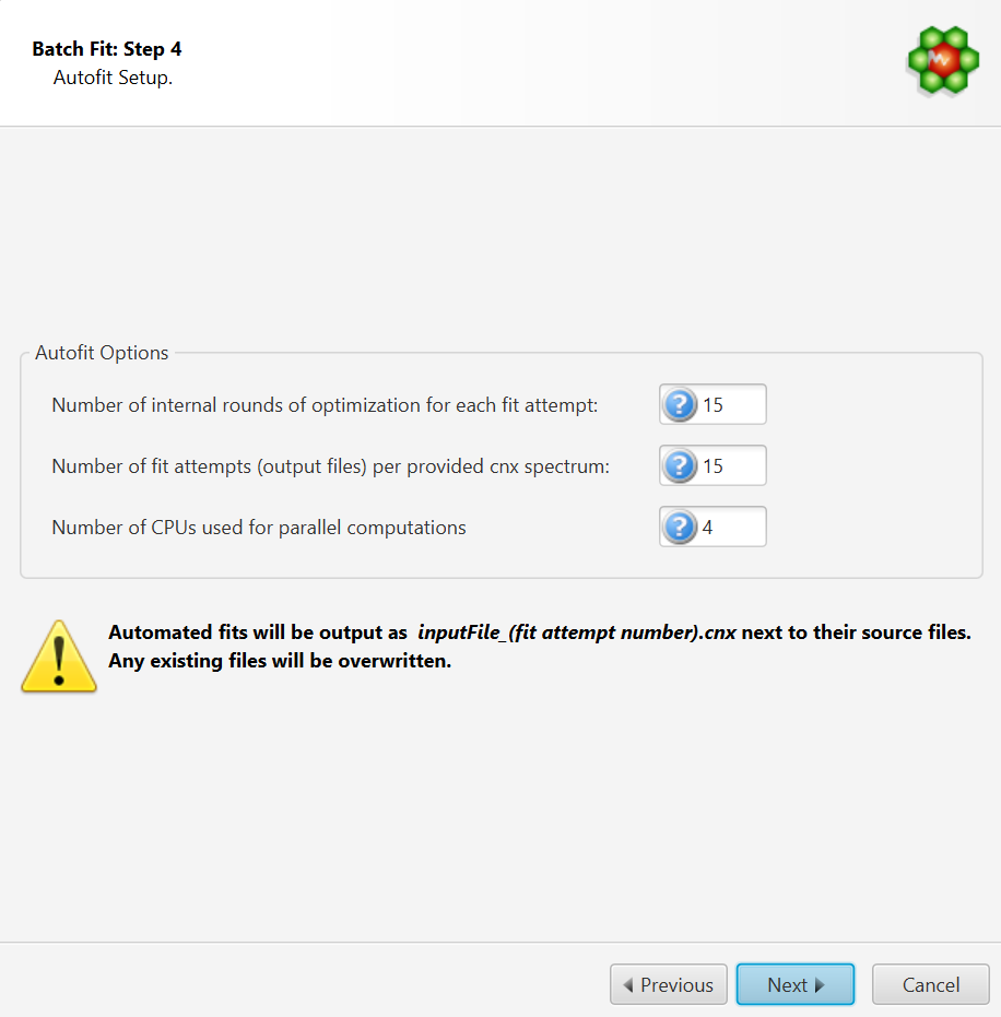
Autofit Setup
This panel controls the overall behaviour of automated fitting:
-
The number of internal iterative rounds is related to the number of times, for each fit attempt of a given spectrum, the algorithm will position clusters and adjust concentrations. It is directly equivalent to the situation encountered with manual fitting, where an operator usually has to do several rounds of going through the list of compounds to be fit and adjust their peak cluster positions and height (concentration).
-
The number of fit attempts control how many output files will be generated for each input spectrum cnx file. By analogy, it is related to how many people would be trying to fit the spectrum if there were a team of operators. Each one could potentially come up with a different solution that produces more or less the same fit quality in terms of sum of squares of the residual line.
-
The number of CPUs control how many CPUs can be used for parallel computations. The number presented in the interface takes into account the maximum number of CPUs allowed and defined by the software license, and the number of CPUs that may already be used by another COMPLETE Autofit job.
-
-
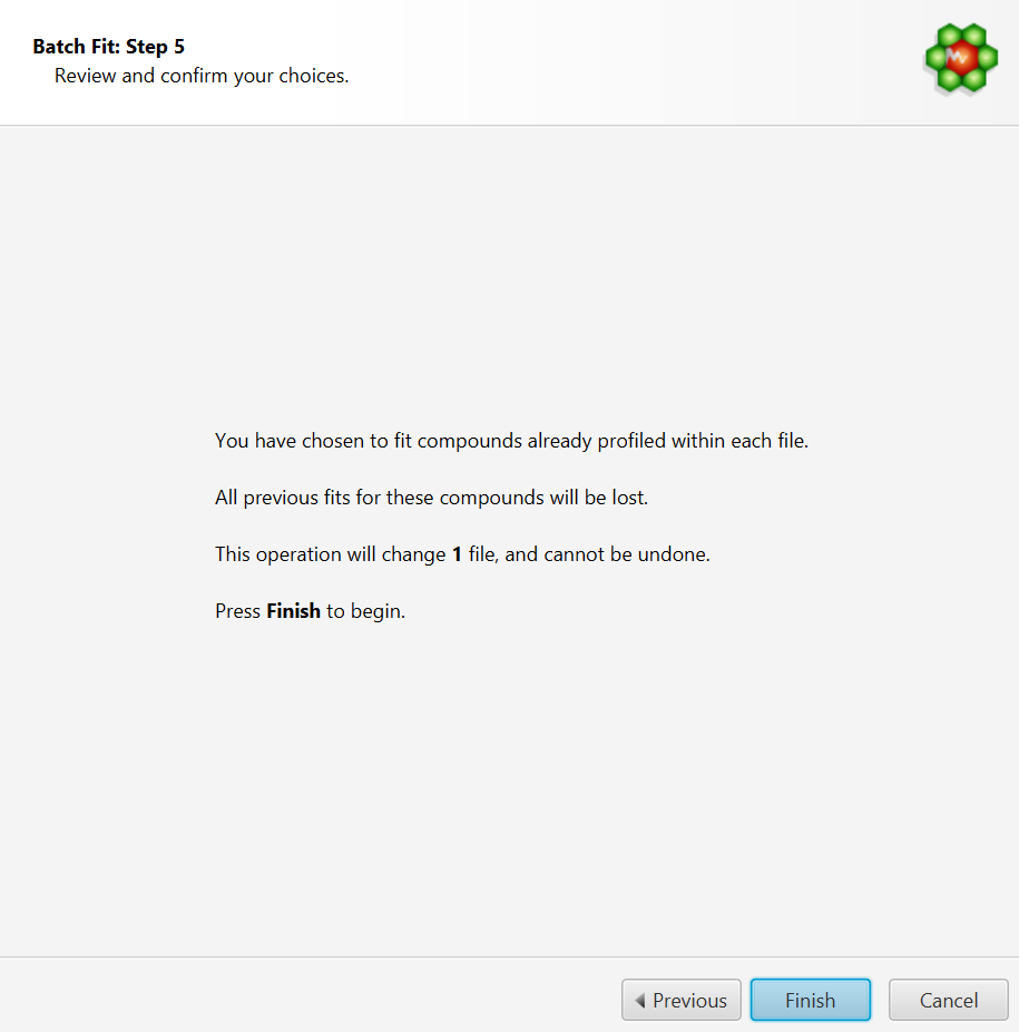
Review and Finish
-
COMPLETE Autofit will generate multiple profiled CNX files for each input spectrum file that will be saved in the same location as the input source. It will not however modify the original source files themselves.
-
A fit report will be produced, showing the residuals chi-square value for each of the produced cnx file. For a given input file, the output solution with the lowest chi square (lowest fit error) is automatically saved with the label “_best” appended at the end of its filename.
-
A text file (.txt) will also be generated for each exported CNX file with the chi square value achieved for each internal round of iteration. Inspection of those text files can reveal whether or not the number of internal rounds that were specified is enough to achieve a minimum. If the best solution (lowest chi square) is generally obtained only at the last internal iterations, it is a sign that maybe a higher number of iterations is needed.
-
It is up to the user to choose the output solution that produced the best fit, if the decision parameter is other than the sum of residuals. For statistical analysis (PCA, PLS-DA, etc.), it may be more relevant to work with concentrations averaged over the series of exported fits rather than single values.
-
Tips and Limitations of COMPLETE Autofit
-
Not all spectra are suitable for automated fitting. Unfiltered spectra showing presence of larger molecules though humps will likely fail. The software does not model the baseline on the fly.
-
The raw fid must be correctly processed and the baseline must be adjusted properly. The software does not model the baseline on the fly.
-
Set the pH for each sample, either in Processor or Profiler. pH information is used to calculate the boundaries for each peak cluster. The software will not fit peak clusters outside of their calculated transform windows.
-
If spectral regions contain intense unknown peaks, exclude those regions from the fit in the provided interface.
-
The time required to fit a spectrum is directly dependant on the number of spectral points, and the total numbers of peak clusters and compounds. Avoid under and over fitting, i.e. work with compound subsets that represent what you should expect to find in the type of samples you are analysing.
A Note about Legacy Autofit
Version 10 also reintroduces a form of automated fitting found in version 8.6 and earlier of the software, as “Legacy Autofit”. Legacy Autofit may be preferable to older users that want to maintain controls for a project initiated using older versions of Chenomx NMR Suite. For users starting a project using Chenomx NMR Suite Versions 9 or later, consider using more advanced Autofit techniques such as Compound Snapper / Fit Automatically or the COMPLETE Autofit Tool.
The difference between Legacy Autofit and COMPLETE Autofit is explained below.
-
Legacy Autofit first takes the raw spectrum and subtracts the contribution of all previously fit compounds that are not selected for the autofit.
-
Starting from the spectrum obtained in step #1, it scores the compounds selected for autofit to establish the order in which they will be fit.
-
Starting from the best potential candidate, it tries to simultaneously establish the position of the clusters for that metabolite and the maximum intensity (and therefore concentration) of that compound on the spectrum. (If it fails to establish where some clusters are located, they are left at their default/untransformed locations.)
-
The contribution of the potential candidate is then subtracted from the spectrum to yield another spectrum which serves as starting point for the processing of the second candidate compound, using the same procedure.
-
This cycle is repeated until the list of selected compounds for autofitting has been exhausted.
-
One can clearly see that the risk of errors increases at every step, and that eventually not all compounds will succeed in being autofitted. Moreover, as individual compounds are added at their maximal concentrations, the final result does not reflect a global optimization of all compounds, but reflects a successive series of individual optimization. (In order words, after adding compound #x, the algorithm does not reevaluate compound #x-1, #x-2, #x-3, etc.)
The main difference between COMPLETE Autofit and the Legacy Autofit approach relies on the fact that the new algorithm is based on a true “global” optimization process. The compound concentrations are obtained altogether (globally) using penalized least squares, rather than through successive fit rounds of individual compounds. The algorithm used for positioning peak clusters has also been greatly improved. Be aware though that there is a computational speed cost to those improvements.