

Manual Profiling can involve a lot of effort in setting compound cluster positions and compound concentrations. Alternatively, you can use a semi-automated approach, or, with the introduction of version 10.0, a fully automated approach.
With the semi-automated approach, the first step consists of positioning compounds clusters on the spectra, followed by an automated concentration optimization based on those positions. Several rounds may be required.
First have Profiler fit cluster postions using the “First Step: Cluster positioning using Compound Snapper” tool and/or compound concentrations using the “Second Step: Concentration optimization using Fit Concentrations” for either the currently selected compound, a selection of compounds, or all compounds in the compound table.
Tips and Tricks
-
Use the Remember Selections feature to the mark compounds that can be reliably Autofit in your project. You can then restore the selection when working on subsequent spectra, allowing you to quickly autofit those compounds.
This feature allows for automatic positioning of peak clusters on the spectrum. It will essentially position peak clusters where their shape best match the experimental spectrum, independent of intensity.
Compound Snapper focuses on optimizing peak cluster locations, individually or in group, depending on the user’s selected cluster(s) or compound(s). Compound Snapper will not attempt to set or modify the concentration of compounds. This functionality automatically positions peak clusters on the spectrum at the location that best matches their global shape. If two or more clusters overlap within their allowed transform window, all possible combinations are analyzed.
As such, this feature is powerful, and will find the proper cluster combination, as sophisticated as it may be, that matches, according to shape, a relevant spectral region.
A snapping operation can either be performed on the original spectral line, or on the subtraction line, i.e. by considering the “left-over” signal from everything that has been fit already. It can also be done on a compound selected in the compound table and whose concentration has not been set already.
How to use Compound Snapper
-
Select one or several clusters from an individual compound, a single or several compounds at once from the compound table, right-click in your selection to bring a contextual menu, or choose 'Snap Compound' from the Compound Menu (main toolbar).
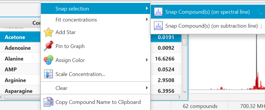
You can also use the keyboard shortcut comma (,) to snap clusters using the experimental spectrum line, or semi-colon (;) to snap clusters using the residual line instead (the residual line is calculated using everything that is already fit except for the clusters/compounds being snapped).
-
To snap all clusters resonating in a particular spectral region at once, first select the region with the Select Region tool (main tool bar), right-click and select “Find and Snap Peak Clusters in this Region”.
Once peak clusters have been positioned, compound concentrations can be fit and optimized using constrained penalized linear least squares, according to:
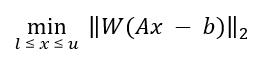
Where...
-
A is the model matrix made up the unscaled individual signatures of the compounds being fit. The current locations of the peak clusters are taken into account when the A matrix is calculated.
-
x is a vector made up all of the compound concentrations to be optimized. Each component of the vector, xi, is bounded between li (lower bound) and ui (upper bound). Non-negative restraints are imposed (li ≥ 0) since concentrations cannot be negative.
-
b is the spectral subtraction line, i.e. the experimental spectrum minus the contribution of all compounds part of the current profile that are not part of the optimization process. In other words, if a compound has been fit and his not part of the fitting process, its contribution is subtracted from the experimental spectrum before the process starts.
-
W is a weight vector, which is used to modulate the relative importance of each spectral point. Optionally, the algorithm can increase the weight of the points that are overfit though an iterative penalization process.
IMPORTANT NOTE: The optimization process will not modify the location of the peak clusters.
How to Fit Automatically
-
Right-click/control-click selected compounds in Profiler’s compound table, or on a selected spectral area.
Concentration Fitting can be performed without a GUI (graphical user interface) by using the Shift+Space bar keyboard shortcut, in which case it uses the default options and values stored in Profiler's preferences.
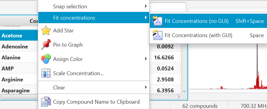
-
Alternatively, temporary settings can be entered via GUI (graphical user interface) using the space bar keyboard shortcut. The interface is composed of three main sections: Regions Selection, Compounds Selection, and Fitting options. The role of each section is described below. The application Preferences panel can be used to control and set all the default values appearing in the interface.
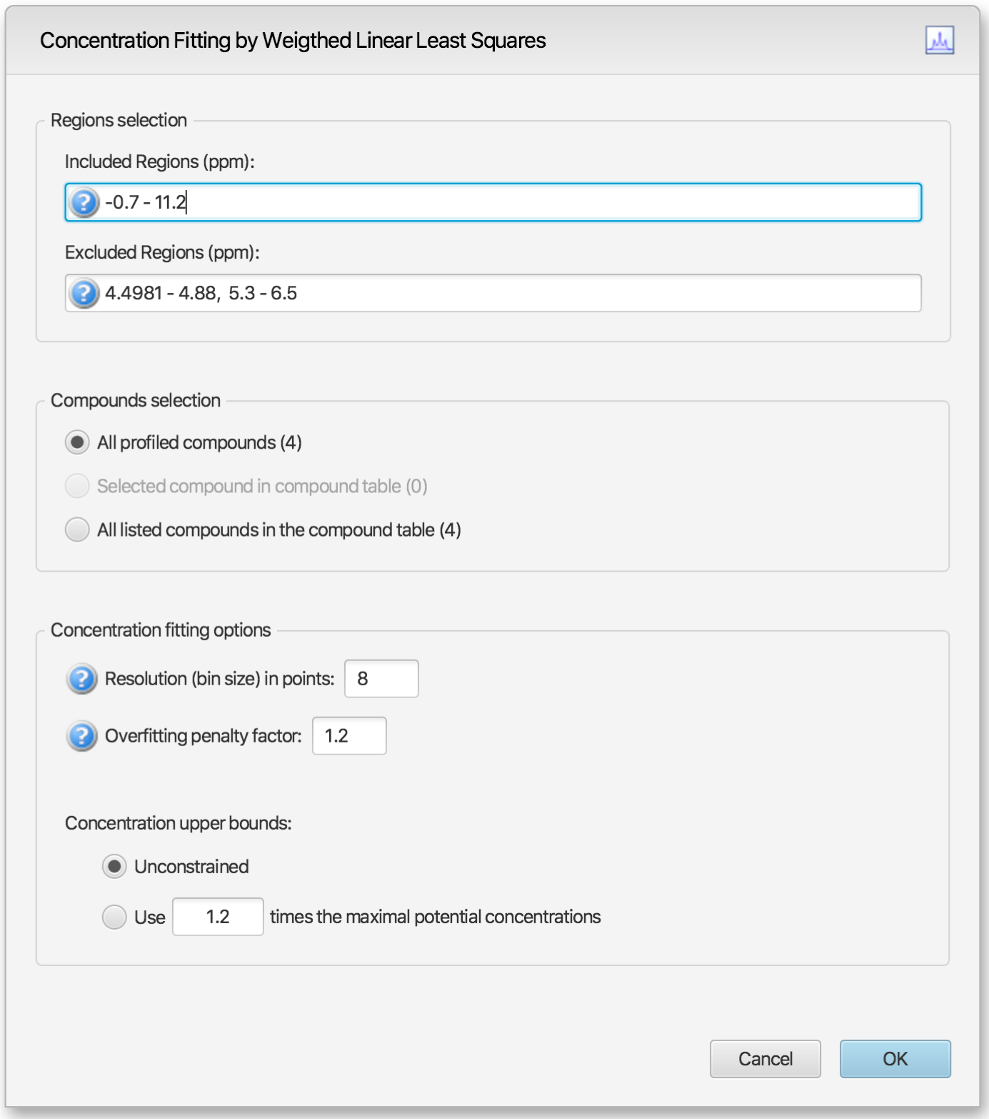
Regions Selection
-
Comma-separated list of spectral regions (in ppm units) to be included or excluded in the fit. Each component of the lists must include a lower and upper bound in ppm, separated by a dash. For instance, “0.8-2.3, 3.0-4.2” is a valid list.
-
The Included Regions input field displays the limits of the currently selected spectral region (as selected with the Select Region Tool), or of the selected clusters for an individual compound. If no region is currently selected, the Included Regions input field defaults to the entire spectrum.
-
The Excluded Regions input field will automatically include the region associated with the water peak. It is recommended that any peaks around the water region be excluded due to attenuation caused by water saturation. Similarly, the region associated with urea (5.4-6.0 ppm) should also be excluded if urea is present.
-
Excluded regions have prevalence over any included regions, i.e. any spectral point falling within any of the listed excluded regions will automatically be ignored during the fit.
Compound Selections
-
Users can optimize either all of the members of the current profile, all of the currently selected compounds in the compound table, or all of the currently listed compounds in the compound table. Note that compounds that do not have a single peak cluster within the participating spectral regions will not be considered for the fit. Their concentrations will not be changed.
Concentration Fitting Options
This group of options control the behavior of the optimization engine.
-
Resolution (bin size): The spectrum can be fit using either its full representation, or a binned representation of it. This parameter controls the number of spectral points per bin. Set this parameter to 1 for full resolution. However, it is highly recommended to use a binned representation if the peak cluster positions have not been optimized. Fitting at full resolution will require more memory and CPU time.
-
Overfitting penalty factor: The amount of overfitting can be limited by increasing the weights of the spectral points where overfitting occurs. This will effectively increase the importance of the spectral points where this occurs relative to the other ones, adding a penalty to pay for predicting points over the spectrum line. For a given spectral point, the square of the difference between the experimentally observed spectrum intensity and the predicted/calculated one will be multiplied by the factor specified in this field if the difference is negative. The weights are adjusted iteratively and up to 5 cycles of optimizations are performed if the specified penalty factor is >1.0.
-
Upper constraints: Non-negative constrained are used during the optimization process so that concentration values remain ≥ 0. Two different settings are offered to control their upper bounds. They can be set to be unlimited via the Unconstrained option, or limited according to their predetermined maximal potential concentration. The maximal potential concentration of a given compound is the highest concentration for which the compound signature would not exceed the experimental spectrum. Because of possible discrepancies between the compound library signatures and the experimental spectrum, mainly due to pH conditions, matrix effects, etc, the potential concentrations determined by Profiler may not be optimal and should only be regarded as guidelines. To give potential concentrations more wiggle room, potential concentrations can be pre-multiplied by a specified constant. The derived set of scaled potential concentration values will then be used as upper bounds.
IMPORTANT NOTE: The baseline is not modeled from the residuals at any stage. It is therefore crucial that the baseline be properly corrected prior to concentration fitting.
Related Topics